Over the last few weeks, Microsoft has focused on improving automation, compatibility, and productivity in Excel for Windows, Mac, and the web. Here are five new features to look out for this month.
1
Automatically Refresh Your PivotTables
Prerequisites |
PivotTables are available in Excel for Microsoft 365, Excel for the web, Excel for Windows (2016 or later), Excel for Mac (2021 or later), and one-off versions of Excel (2016 or later). However, you must be using the latest versions of Excel for Windows or Mac to access the new Auto Refresh feature. |
|---|---|
Availability | PivotTable Auto Refresh is currently in the testing phase with members of the Microsoft Insider program using Excel for Windows Version 2506 (Build 19008.2000) or later or Excel for Mac Version 16.99 (Build 250616106) or later. It is expected to become available to everyone using desktop versions of Excel in the coming months. |
PivotTables are one of the most powerful features in Microsoft Excel, allowing you to organize and analyze large datasets in a condensed and intuitive way. However, one problem has always been that they don’t refresh automatically if the source data changes, meaning you could inadvertently be working with outdated figures.
The addition of the Auto Refresh tool means that any updates to the source range are instantly reflected in the corresponding PivotTable.
What’s more, Auto Refresh is now the default state for all PivotTables in Excel. To turn it off (or back on again), select a cell in the PivotTable, and click “Auto Refresh” in the PivotTable Analyze tab on the ribbon.
When Auto Refresh is turned off, an indicator is added to the status bar in the bottom-left corner of the Excel window to let you know that the PivotTables are pulling out-of-date data. Click this indicator to force an immediate refresh.
PivotTable Auto Refresh only works when the source data is in the same workbook as the PivotTable itself, and you can’t activate this capability if the PivotTable contains external or asynchronous data. It may also be unavailable if you’re working on a spreadsheet at the same time as someone else who is using an older version of Excel, or if the source data contains volatile functions, like RAND or NOW.
Read More: Microsoft
2
Switch to Different Compatibility Versions for Improved Text Functions
Prerequisites |
You must be using Excel for Windows, Mac, or the web to see the new Compatibility Version tool. |
|---|---|
Availability | This feature is currently transitioning from an Insider-only tool to general availability, so if you don’t have it yet, you’ll see it soon. |
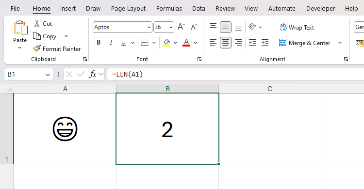
If you’ve ever tried to use Excel’s text functions—LEN, MID, SEARCH, FIND, and REPLACE—in formulas referencing cells with Unicode characters—like symbols or emojis—you will have noticed that they double-count them.
For example, here, typing:
=LEN(A1)
into cell B1 returns 2, even though there’s only one character in cell A1.
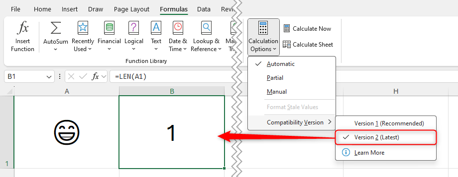
However, thanks to this update, the text functions now only count each character once. But (and it’s a big but), there’s a step you have to take before you can see it in action.
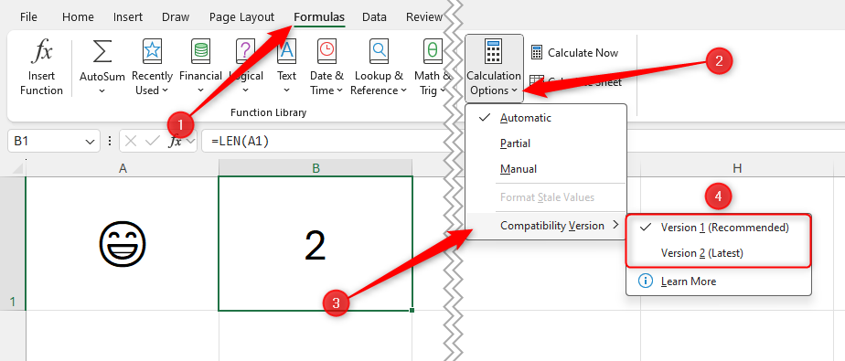
So that this function update doesn’t affect existing formulas in all your other workbooks, Microsoft has rolled it out as a separate compatibility version. Head to the “Formulas” tab on the ribbon, and click “Calculation Options.” Then, when you hover over “Compatibility Version,” you’ll see two options: Version 1 and Version 2.
Existing spreadsheets are currently set to Version 1 by default, which, when selected, reflects the historical calculation behavior. This is currently the recommended version, as it means that your spreadsheet will be compatible with older versions of Excel.
If someone opens a spreadsheet that is set to a version they can’t currently access, they will see a warning that the calculation results may be inconsistent.
However, if you switch your spreadsheet to Version 2, you’re activating the new calculation rollout, meaning the text functions only count Unicode characters once.
Changing the compatibility version in Microsoft Excel only affects the active workbook.
Once rollout is complete, new workbooks will adopt Version 2 by default. Microsoft anticipates that this will be around January 2026.
Read More: Microsoft
3
Connect to External Data With the New Get Data Window
Prerequisites |
Although the traditional Get Data drop-down menu comes as standard in the latest versions of Excel for Windows and Mac, you must be using Excel for Windows to see the new Get Data window. |
|---|---|
Availability | This feature is currently in the preview phase for members of the Microsoft Insider program using Excel for Windows Version 2505 (Build 18829.20000). It is expected to become available to everyone using Excel for Windows in the coming months, though there’s no word from Microsoft on when those using Excel for Mac will receive it. |
Microsoft Excel’s Get Data functionality lets you import data from various sources—like CSVs, websites, or other workbooks—into your spreadsheet. You can then use the Power Query Editor to clean up and transform the imported data.
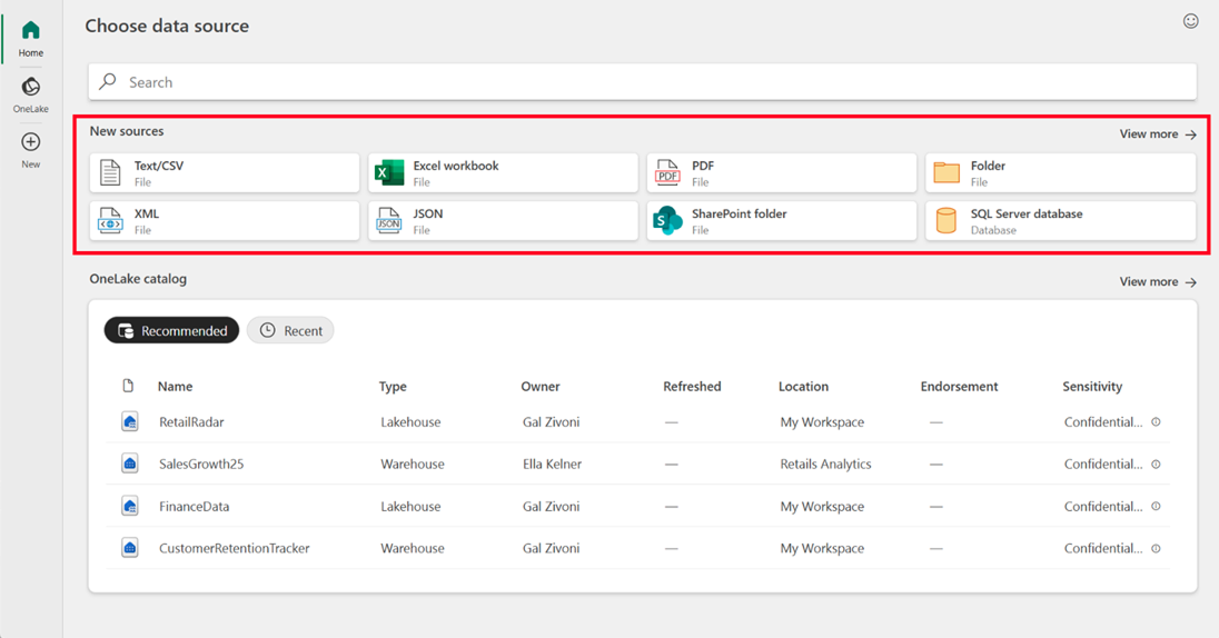
Microsoft has now modernized this tool in Excel for Windows with a brand-new interface and the option to import data from your organization’s OneLake catalog.
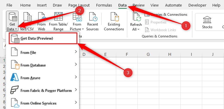
To access it, open the “Data” tab on the ribbon, and click the “Get Data” down arrow. Then, click “Get Data (Preview).”
Once this update is made generally available, clicking the “Get Data” button is likely to open a new window rather than trigger a drop-down menu.
Then, choose one of the various ways to import data into your Excel file.
To see more options, click “New” in the left-hand sidebar. On the other hand, if you’re logged in to an organization account, click “OneLake” to browse your OneLake catalog.
Read More: Microsoft
4
See More Than One Worksheet Side by Side in Excel for Mac
Prerequisites |
You must be using Excel for Mac or Excel for Windows to see this feature. |
|---|---|
Availability | Those using Excel for Windows have been able to access the Side By Side tool for some time. This update brings it into general circulation for those using Excel for Mac Version 16.97 (Build 25041535) or later. However, the tool is not currently available in Excel for the web or the Excel mobile app. |
The New Window View in Microsoft Excel (accessed via the View tab on the ribbon) is a great way to see two or more parts of a file simultaneously, saving you from having to scroll back and forth or constantly flick between two or more tabs.
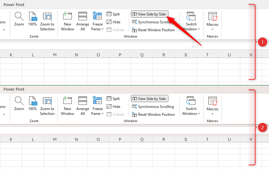
In Excel for Windows, after clicking “New Window,” the option to arrange the various windows side-by-side becomes active, meaning you can easily compare the data in each view.
Click “Arrange All” in the View tab to switch between horizontal, vertical, and tiled side-by-side views. Also, to scroll up and down all duplicated windows at the same time, click “Synchronous Scrolling.”
However, before this update, if you wanted to achieve the same side-by-side view in Excel for Mac, after clicking “New Window,” you would have to click and drag the windows manually to arrange them.
Now, those using Excel for Mac have the same single-click side-by-side functionality as those using Excel for Windows.
Read More: Microsoft
5
Refresh Power Query in Excel for the Web With Authenticated Data Sources
Prerequisites |
You must be using Excel for Windows, Mac, or the web to take advantage of this Power Query capability. A desktop version of Excel must be used to import data into a spreadsheet, but you can then view data connections and work with existing queries in Excel for the web. |
|---|---|
Availability | This tool is now generally available to those using Excel for the web. Those using Excel for Windows or Mac have been able to use this feature for some time. |
Previously, you could only refresh Power Query in Excel for the web when data was imported from within the existing workbook or anonymous OData feeds. However, now, you can also refresh Power Query data sourced from authenticated data sources, like organizational SharePoint or OneDrive folders, an Azure table, or Microsoft Exchange Online.
Even though the data source connections have been updated, the process for updating them is the same. In the Data tab on the ribbon, click “Refresh” to update the active table or “Refresh All” to update everything.
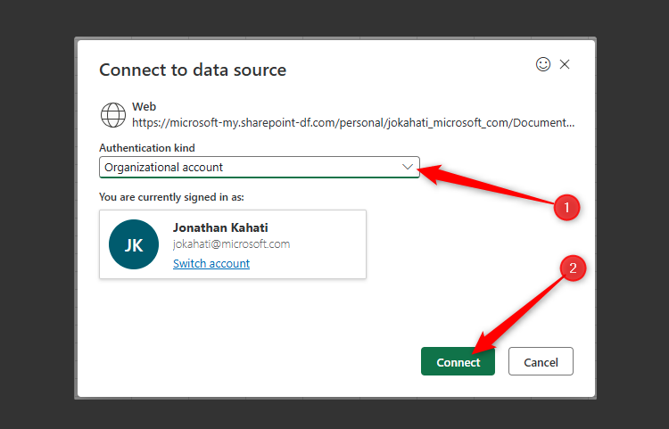
At this point, you may need to provide authentication. To do this, select the relevant method in the Connect To Data Source dialog box—”Anonymous,” “User And Password,” or “Organizational Account.” Then, once you’ve been identified, click “Connect.”
Microsoft says that future plans include releasing the entire Power Query Editor functionality to Excel for the web, but there’s no word on when this will happen.
Read More: Microsoft
To access all the best features of the Microsoft programs—including the desktop versions, enhanced security, and the ability to work on several devices—sign up for a Microsoft 365 account.


